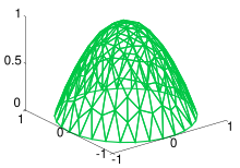
In applied mathematics, discretization is the process of transferring continuous functions, models, variables, and equations into discrete counterparts. This process is usually carried out as a first step toward making them suitable for numerical evaluation and implementation on digital computers. Dichotomization is the special case of discretization in which the number of discrete classes is 2, which can approximate a continuous variable as a binary variable (creating a dichotomy for modeling purposes, as in binary classification).

Discretization is also related to discrete mathematics, and is an important component of granular computing. In this context, discretization may also refer to modification of variable or category granularity, as when multiple discrete variables are aggregated or multiple discrete categories fused.
Whenever continuous data is discretized, there is always some amount of discretization error. The goal is to reduce the amount to a level considered negligible for the modeling purposes at hand.
The terms discretization and quantization often have the same denotation but not always identical connotations. (Specifically, the two terms share a semantic field.) The same is true of discretization error and quantization error.
Mathematical methods relating to discretization include the Euler–Maruyama method and the zero-order hold.
Discretization of linear state space models
editDiscretization is also concerned with the transformation of continuous differential equations into discrete difference equations, suitable for numerical computing.
The following continuous-time state space model
where v and w are continuous zero-mean white noise sources with power spectral densities
can be discretized, assuming zero-order hold for the input u and continuous integration for the noise v, to
with covariances
where
and T is the sample time. If A is nonsingular,
The equation for the discretized measurement noise is a consequence of the continuous measurement noise being defined with a power spectral density.[1]
A clever trick to compute Ad and Bd in one step is by utilizing the following property:[2]: p. 215
Where Ad and Bd are the discretized state-space matrices.
Discretization of process noise
editNumerical evaluation of Qd is a bit trickier due to the matrix exponential integral. It can, however, be computed by first constructing a matrix, and computing the exponential of it[3] The discretized process noise is then evaluated by multiplying the transpose of the lower-right partition of G with the upper-right partition of G:
Derivation
editStarting with the continuous model we know that the matrix exponential is and by premultiplying the model we get which we recognize as and by integrating, which is an analytical solution to the continuous model.
Now we want to discretise the above expression. We assume that u is constant during each timestep. We recognize the bracketed expression as , and the second term can be simplified by substituting with the function . Note that . We also assume that u is constant during the integral, which in turn yields
which is an exact solution to the discretization problem.
When A is singular, the latter expression can still be used by replacing by its Taylor expansion, This yields which is the form used in practice.
Approximations
editExact discretization may sometimes be intractable due to the heavy matrix exponential and integral operations involved. It is much easier to calculate an approximate discrete model, based on that for small timesteps . The approximate solution then becomes:
This is also known as the Euler method, which is also known as the forward Euler method. Other possible approximations are , otherwise known as the backward Euler method and , which is known as the bilinear transform, or Tustin transform. Each of these approximations has different stability properties. The bilinear transform preserves the instability of the continuous-time system.
Discretization of continuous features
editIn statistics and machine learning, discretization refers to the process of converting continuous features or variables to discretized or nominal features. This can be useful when creating probability mass functions.
Discretization of smooth functions
editIn generalized functions theory, discretization arises as a particular case of the Convolution Theorem on tempered distributions
where is the Dirac comb, is discretization, is periodization, is a rapidly decreasing tempered distribution (e.g. a Dirac delta function or any other compactly supported function), is a smooth, slowly growing ordinary function (e.g. the function that is constantly or any other band-limited function) and is the (unitary, ordinary frequency) Fourier transform. Functions which are not smooth can be made smooth using a mollifier prior to discretization.
As an example, discretization of the function that is constantly yields the sequence which, interpreted as the coefficients of a linear combination of Dirac delta functions, forms a Dirac comb. If additionally truncation is applied, one obtains finite sequences, e.g. . They are discrete in both, time and frequency.
See also
editReferences
edit- ^ Analytic Sciences Corporation. Technical Staff. (1974). Applied optimal estimation. Gelb, Arthur, 1937-. Cambridge, Mass.: M.I.T. Press. pp. 121. ISBN 0-262-20027-9. OCLC 960061.
- ^ Raymond DeCarlo: Linear Systems: A State Variable Approach with Numerical Implementation, Prentice Hall, NJ, 1989
- ^ Charles Van Loan: Computing integrals involving the matrix exponential, IEEE Transactions on Automatic Control. 23 (3): 395–404, 1978
Further reading
edit- Robert Grover Brown & Patrick Y. C. Hwang (1997). Introduction to random signals and applied Kalman filtering (3rd ed.). ISBN 978-0471128397.
- Chi-Tsong Chen (1984). Linear System Theory and Design. Philadelphia, PA, USA: Saunders College Publishing. ISBN 978-0030716911.
- C. Van Loan (Jun 1978). "Computing integrals involving the matrix exponential" (PDF). IEEE Transactions on Automatic Control. 23 (3): 395–404. doi:10.1109/TAC.1978.1101743. hdl:1813/7095.
- R.H. Middleton & G.C. Goodwin (1990). Digital control and estimation: a unified approach. Prentice Hall. p. 33f. ISBN 978-0132116657.