File:Helmholtz coil, B magnitude cross section.svg

Original file (SVG file, nominally 540 × 540 pixels, file size: 250 KB)

Summary

Description
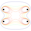
English: Cross section of B (magnetic field strength) magnitude in a Helmholtz coil (actually consisting of two coils: one at the top, one at the bottom in the plot). The eight contours are for field magnitudes of 0.5 B0, 0.8 B0, 0.9 B0, 0.95 B0, 0.99 B0, 1.01 B0, 1.05 B0, and 1.1 B0, where B0 is field strength at center. The large center area has almost uniform field strength.
Date
Source Own work
Author Morn

Licensing

I, the copyright holder of this work, hereby publish it under the following licenses:
w:en:Creative Commons
attribution share alike
This file is licensed under the Creative Commons Attribution-Share Alike 3.0 Unported license.
You are free:
  • to share – to copy, distribute and transmit the work
  • to remix – to adapt the work
Under the following conditions:
  • attribution – You must give appropriate credit, provide a link to the license, and indicate if changes were made. You may do so in any reasonable manner, but not in any way that suggests the licensor endorses you or your use.
  • share alike – If you remix, transform, or build upon the material, you must distribute your contributions under the same or compatible license as the original.
GNU head Permission is granted to copy, distribute and/or modify this document under the terms of the GNU Free Documentation License, Version 1.2 or any later version published by the Free Software Foundation; with no Invariant Sections, no Front-Cover Texts, and no Back-Cover Texts. A copy of the license is included in the section entitled GNU Free Documentation License.
You may select the license of your choice.

Python source code

from pylab import *    # needs Matplotlib

r = 1
res = 500	# grid resolution (100 seems to be sufficient here and will create a smaller SVG file)
figure(figsize=(6, 6))
axes((0,0,1,1), frameon = False)

def dist3(a,b,c,d,e,f):
	return maximum(r, sqrt((a-d)**2 + (b-e)**2 + (c-f)**2))

x = linspace(-150, 150, res)
y = linspace(-150, 150, res)
X,Y = meshgrid(x,y)
F = zeros((res,res,3))

# loop over two coils
for coils in 1,-1:
	# sum field contributions from coil in 10-degree steps
	for p in range(0, 360, 10):
		xc,yc,zc = (100*sin(pi*p/180),50*coils,100*cos(pi*p/180))
		MAG = 1/((r+dist3(X,Y,0,xc,yc,zc))**3)
		# (We leave out the necessary constants that would be required
		# to get proper units because only scaling behavior will be shown
		# in the plot. This is also why a sum instead of an integral
		# can be used.)
		Z = cross((X[:,:,newaxis]-xc,Y[:,:,newaxis]-yc,-zc),(-zc,0,xc))
		F += Z[0,:,:]*MAG[:,:,newaxis]

B = sqrt(F[:,:,0]**2+F[:,:,1]**2+F[:,:,2]**2)
# scale field strength by value at center:
B = B / B[res/2,res/2]

contour(x,y,B, levels = (.5,.8,.9,.95,.99,1.01,1.05,1.1))

# add wire symbols:
scatter((100,100,-100,-100), (50,-50,50,-50), s = 400, color = "black")

axis((-130, 130, -130, 130))
xticks([])
yticks([])

savefig("Helmholtz_coil,_B_magnitude_cross_section.svg")

show()

Captions

Add a one-line explanation of what this file represents

Items portrayed in this file

depicts

13 May 2014

File history

Click on a date/time to view the file as it appeared at that time.

Date/TimeThumbnailDimensionsUserComment
current00:09, 13 May 2014Thumbnail for version as of 00:09, 13 May 2014540 × 540 (250 KB)Morn{{Information |Description ={{en|1=Cross section of B magnitude in a Helmholtz coil (actually consisting of two coils, one at the top, one at the bottom in the plot). Field strength is scaled by center value, isolines are at .5,.8,.9,.95,.99,1.01,1....

The following page uses this file:

Global file usage

The following other wikis use this file:

Metadata